Updated November 3, 2026. A method note on validation splits and selection bias. Code and numbers are illustrations on randomly generated data, not investment results from any real strategy.
Read a good backtest number together with the number of trials
Run hundreds of parameter combinations over the same period and keep the best one, and one of them will tend to look good even when none has a real edge. Bailey, Borwein, López de Prado, and Zhu (2014) point out that when the number of configurations tried is large relative to the available history, the best-looking backtest can simply be fitted to chance extremes in the sample.
The example below creates 200 hypothetical strategies with zero expected return and selects the one with the highest Sharpe ratio over the first 252 observations.
import numpy as np

rng = np.random.default_rng(7)
n_trials, n_is, n_oos = 200, 252, 252

# 200 hypothetical strategies with zero expected return: none has a real edge
returns = rng.normal(0.0, 0.01, size=(n_trials, n_is + n_oos))
is_ret, oos_ret = returns[:, :n_is], returns[:, n_is:]

def sharpe(r):
    return r.mean(axis=-1) / r.std(axis=-1, ddof=1)

is_sharpe = sharpe(is_ret)
best = int(np.argmax(is_sharpe))

# The standard error of a Sharpe estimate is roughly 1/sqrt(T) (per observation, not annualized)
se = 1 / np.sqrt(n_is)
print(f"best in-sample SR: {is_sharpe[best]:.3f}, SE ~ {se:.3f}")
print(f"same strategy out-of-sample SR: {sharpe(oos_ret[best]):.3f}")

assert abs(is_sharpe.mean()) < se                # on average there is no edge
assert is_sharpe[best] > 2 * se                  # picking only the best makes one appear
assert sharpe(oos_ret[best]) < is_sharpe[best]   # the same strategy falls back in the next period
With this seed the selected strategy’s in-sample Sharpe is about 2.8 standard errors, and it is negative in the following period. The structure matters more than the numbers: however carefully you split the data, failing to adjust for having picked the maximum of many candidates inflates the result.
Walk-forward replays the operating sequence but yields few test periods
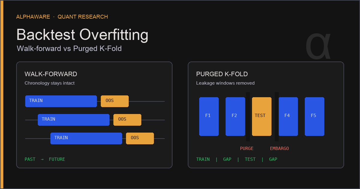
Walk-forward fits parameters on a past window, evaluates on the period immediately after, then rolls the window forward and repeats. Its strength is that it follows the same order of events as live operation.
scikit-learn’s TimeSeriesSplit provides this structure as an expanding window. In the k-th split it uses the first k folds for training and the next fold for testing, and each training set contains the previous ones. max_train_size caps the training window, and gap is the number of samples excluded from the end of each training set before the test set.
If the label is a forward return, set gap to at least the label horizon so that every training label is fully realized before the test period starts.
import numpy as np
from sklearn.model_selection import TimeSeriesSplit

n, horizon = 120, 5
start = np.arange(n)                          # decision time i
end = np.minimum(start + horizon, n - 1)      # time at which the label is realized

tscv = TimeSeriesSplit(n_splits=4, test_size=20, gap=horizon)
for train_idx, test_idx in tscv.split(start):
    # with gap >= label horizon, training labels are realized before the test period starts
    assert end[train_idx].max() < test_idx.min()
    assert train_idx.max() + horizon < test_idx.min()
The cost is data. Each observation is tested at most once, and the earliest segment is never tested. With few test periods it is hard to estimate the dispersion of results, and a single market regime can dominate the outcome.
When labels overlap, a chronological split alone still leaks
Ordinary k-fold trains on data both before and after the test fold. In financial data the more specific problem is overlapping label windows. If the label at time t is the return from t+1 to t+5, training samples just before the test fold have labels built from the same price moves as the test fold.
Chapter 7 of López de Prado’s Advances in Financial Machine Learning (2018) proposes two devices.
- Purging: remove training samples whose label-formation window overlaps the test labels’ window. The decision uses each sample’s label start and end times, not simply “a few neighboring rows”.
- Embargo: also drop a fixed number of samples immediately after the test period. It is a buffer against links that label overlap alone does not catch, such as serial correlation in features.
import numpy as np

def purged_kfold(start, end, n_splits=5, embargo=0):
    """Drop training samples whose label window [start[i], end[i]] overlaps the test window,
    and drop `embargo` samples right after the test labels end."""
    idx = np.arange(len(start))
    for test_idx in np.array_split(idx, n_splits):
        test_start = start[test_idx].min()
        test_end = end[test_idx].max()
        overlap = (start <= test_end) & (end >= test_start)
        after = (start > test_end) & (start <= test_end + embargo)
        train_idx = idx[~overlap & ~after]
        yield train_idx, test_idx

n, horizon, embargo = 120, 5, 3
start = np.arange(n)
end = np.minimum(start + horizon, n - 1)

for train_idx, test_idx in purged_kfold(start, end, n_splits=5, embargo=embargo):
    t0, t1 = start[test_idx].min(), end[test_idx].max()
    # 1) no training label window overlaps the test label window
    assert not np.any((start[train_idx] <= t1) & (end[train_idx] >= t0))
    # 2) the embargo window right after the test labels is not in training
    assert not np.any((start[train_idx] > t1) & (start[train_idx] <= t1 + embargo))
    # 3) samples after the test period are still used: the difference from a chronological split
    if t1 + embargo < n - 1:
        assert start[train_idx].max() > t1
The third condition shows what the method is. Purged k-fold also trains on data after the test period. It blocks label leakage, but it is not a replay of “training only on what was known at the time”. That difference matters when market structure changes over time.
The two methods are not substitutes; they answer different questions
| Criterion | Walk-forward | Purged k-fold |
|---|---|---|
| Question answered | How would it have done if run in order | Does the model generalize without label leakage |
| Number of test periods | Few; each observation tested at most once | Many; every fold is tested once |
| Trains on later data | No | Yes, includes samples after the test period |
| Information needed | Training window length, gap |
Per-sample label start and end times, embargo length |
| Watch out for | One regime can dominate | Structural change over time can be averaged away |
A common sequence is to narrow model and hyperparameter candidates with purged k-fold, then check the final choice with walk-forward on an untouched recent period. Similar results from both do not prove the absence of overfitting, though. If you kept revising candidates while looking at the same data, both validations carry the effect of that selection process.
The split method does not fix selection bias
Bailey and López de Prado’s (2014) Deflated Sharpe Ratio (DSR) aims to correct two sources of inflation: selection bias from testing many strategies and keeping the best, and distortion from non-normal returns. Its starting point is that the expected maximum Sharpe ratio obtained by luck alone rises as more alternatives are tested.
Computing the DSR requires the number of trials and the variance of Sharpe ratios across them. So record-keeping comes before the formula.
- Log every parameter combination, feature set, and period definition you tested, including the ones discarded for poor results.
- Decide how to group near-identical strategies so they are not counted as independent trials.
- Once you choose a final candidate, do not change rules after looking at the test period again. If you do, add that to the trial log too.
Conditions to check before trusting the performance table
These are conditions to test before believing a result. It is better to set pass criteria before seeing the results.
- In-sample versus out-of-sample gap: a large drop in test performance points to selection bias or structural change. Look at the distribution across several periods rather than one.
- Parameter sensitivity: check whether neighboring parameters around the optimum give similar results. A result that is good at only one point is likely fitted to chance.
- Signal and execution timing: assuming a signal built from the close fills at that same close is a common lookahead. Separate when a signal is confirmed from when an order can be placed.
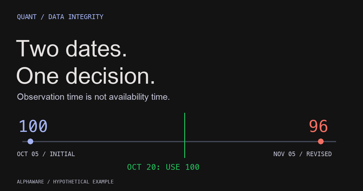
- Data availability time: for revised indicators, use the version available at the time. See the point-in-time data article.
- Trading costs and slippage: the higher a strategy’s turnover, the more sensitive the result is to cost assumptions. Vary the costs and see how the result changes.
Sources and scope
- Bailey, Borwein, López de Prado, Zhu (2014), Notices of the AMS 61(5): backtest overfitting when trials outnumber the available data.
- Bailey & López de Prado (2014), The Deflated Sharpe Ratio, Journal of Portfolio Management 40(5): a Sharpe ratio corrected for selection bias and non-normality.
- López de Prado (2018), Advances in Financial Machine Learning, Wiley: Chapter 7 on purging and embargo in financial cross-validation.
- scikit-learn TimeSeriesSplit: expanding-window splits,
max_train_size, andgap. - This article describes validation procedures only; it does not claim that a strategy passing any split method or checklist will be profitable in live trading.